Spin defects in hexagonal boron nitride

Diamond NV centers made quantum sensing practical, but they sit inside a bulk crystal, which limits how close they get to a sample. VB⁻ lives in a van der Waals material that can be thinned to a few layers and stacked directly onto other 2D materials. Its ground state is a spin triplet, described by

At zero field the $m_s = \pm 1$ levels sit about 3.48 GHz above $m_s = 0$. The two levels differ in how brightly the defect fluoresces, so sweeping a microwave drive across the resonance shows up as a dip in photoluminescence. A magnetic field along the c-axis splits that dip into two:

Reading the splitting gives the local field. Strain and temperature move $D$, which turns the same defect into a sensor for those too. None of that matters until the defects exist in the right density, which is where my work starts.

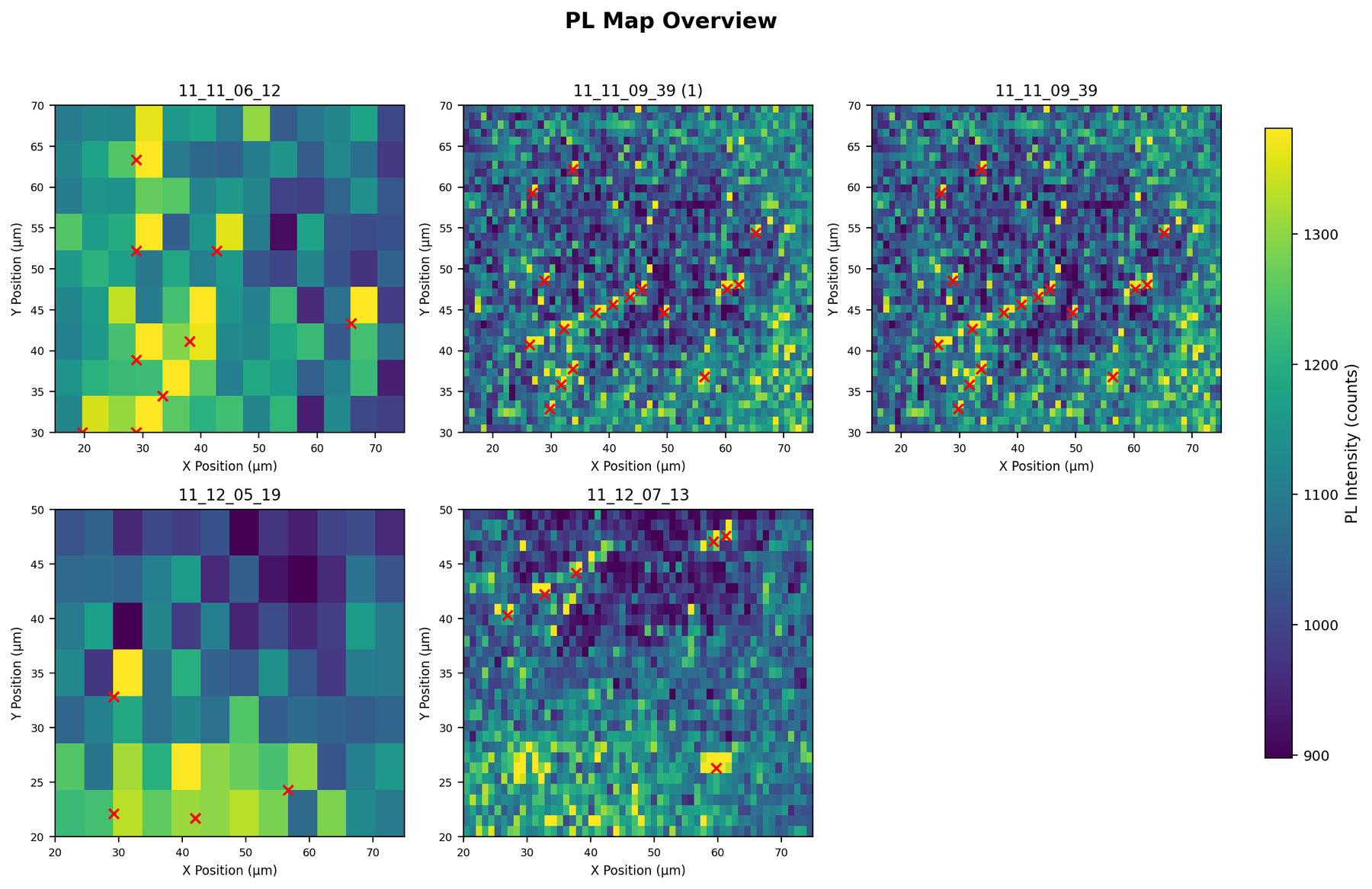
Boron vacancies form when an incoming ion knocks a boron atom out of the lattice. Our first samples were exfoliated hBN flakes on SiO₂/Si, mapped with confocal photoluminescence (PL), irradiated with a 2 MeV ion beam in the Rutherford backscattering (RBS) chamber, and mapped again.

The first trial, a 30-minute exposure, did not raise PL at all. Typical intensities dropped from roughly 120–160 to 70–110 (arbitrary units). The second trial ran for 11 hours. Afterward the maps showed isolated bright spots that stayed in the same places across repeated scans, which rules out transient noise. The overall comparison is mixed: a few irradiated maps are far brighter than anything before dosing, but they contain fewer bright clusters.

PL intensity alone cannot say whether a bright spot is VB⁻ or some other emitter. That needs a spin measurement (§5). Choosing beam energy and dose more deliberately is what the simulation work in §3 is for.

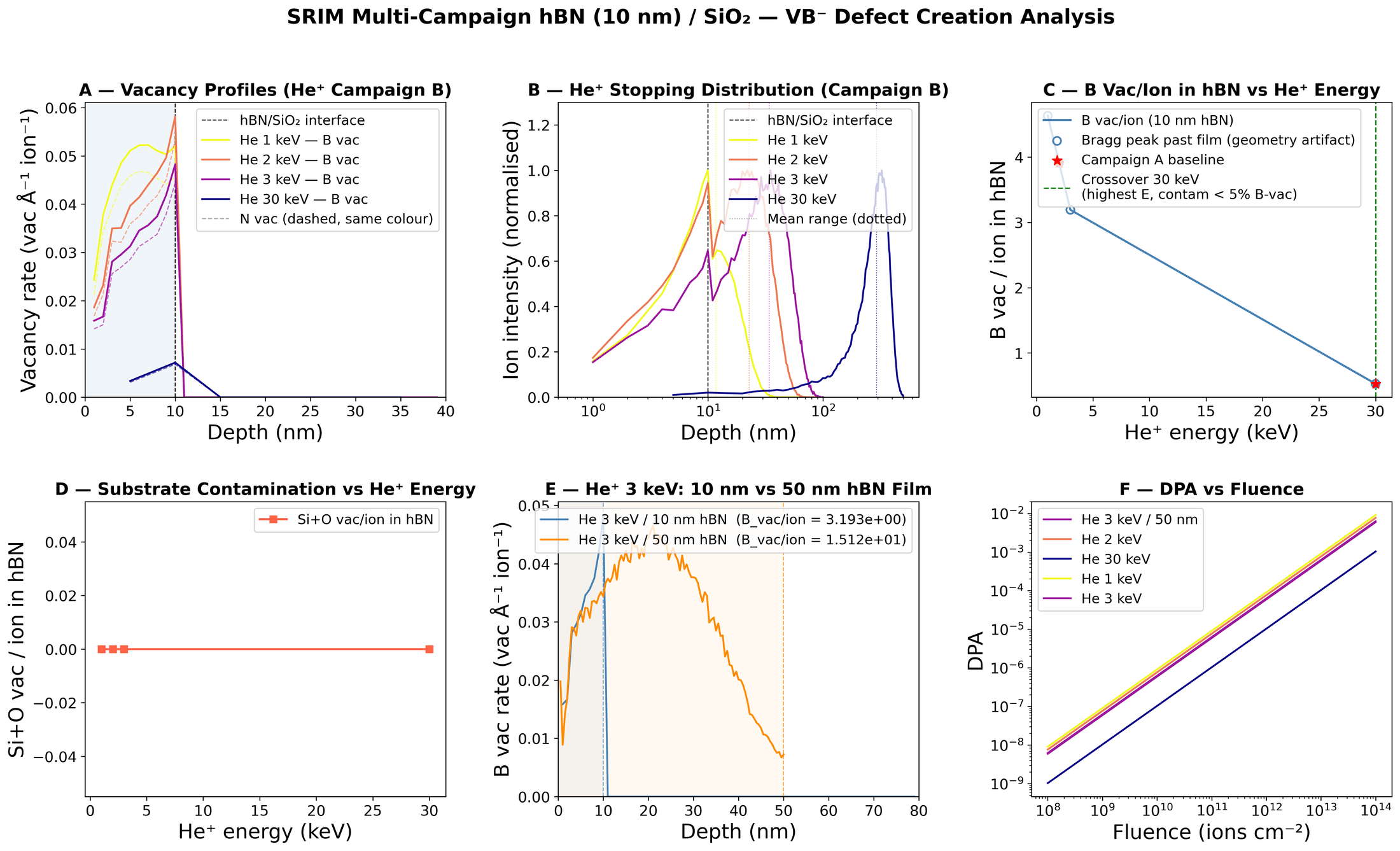
SRIM/TRIM follows individual ions through a target and tallies every displaced atom. I ran four campaigns on a 10 nm hBN film over SiO₂: a helium baseline (A), a helium energy sweep from 1 to 30 keV (B), a proton sweep (C), and a check on whether an ordinary RBS measurement at MeV energies creates unintended vacancies (D). A parser turns the raw SRIM tables into vacancy depth profiles and per-ion yields, then into fluence tables.

For a boron vacancy yield $Y_B$ (vacancies per incident ion inside the film) and boron areal density $N_B$, damage grows linearly with fluence $\Phi$:

The useful results: low-energy helium does most of its damage inside the film. At 3 keV each ion leaves about 3.2 boron vacancies in 10 nm of hBN, while at 30 keV most of the cascade lands in the substrate and the yield falls to about 0.5 (panel C). SRIM shows no substrate contamination of the film anywhere in the sweep (panel D). Film thickness matters: the same 3 keV beam yields 15.1 vacancies per ion in a 50 nm film (panel E). At $10^{14}\ \mathrm{cm^{-2}}$, 3 keV helium reaches about $6\times10^{-3}$ DPA, just under the overdamage line (panel F).

Alongside SRIM I built a classifier that takes an ion, energy, and fluence and places the result in a damage regime: below threshold, sparse, dense, or overdamaged. It also returns the closest matches from a table of about 20 published irradiation experiments. An earlier version also estimated spin observables; the current one reports only the damage regime and the literature matches.

I wrote the analysis code for our PL data. The pipeline crops each map to its real scan area, fits and clusters bright spots, and compares conditions. It replaced a dozen one-off scripts, and every past analysis can now be rerun from raw data with one command. An early version distorted the data in a way that looked fine: I had tuned it to look right before I understood the physics well enough to judge it. The rebuilt version is the one I use now.

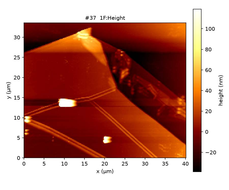
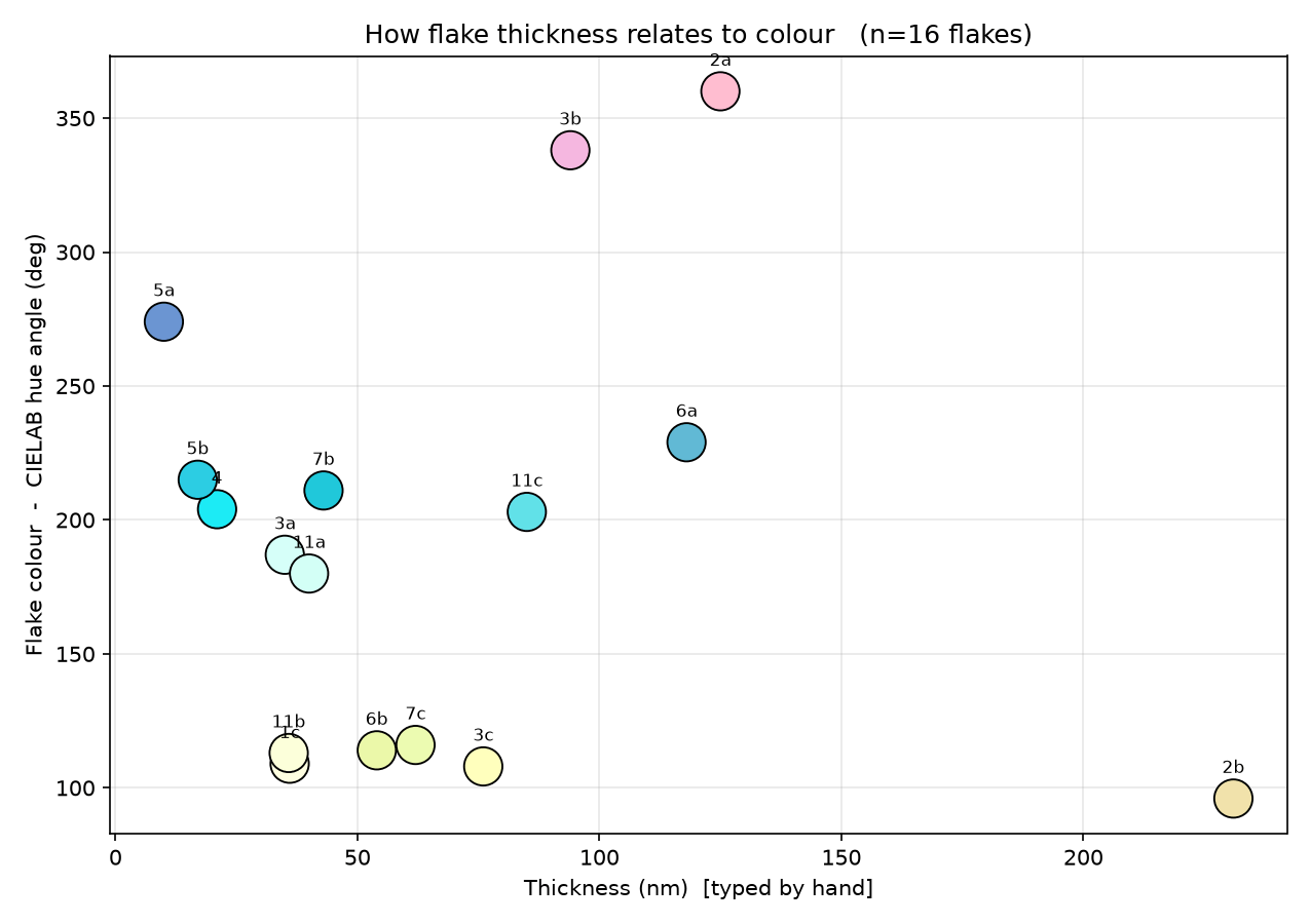
For the July 2026 sample of 23 flakes, between 10 and 231 nm thick, I wrote two bench tools. One overlays PL maps on optical images and averages PL over hand-drawn flake outlines. The other reads NT-MDT .mdtAFM files directly, with no Gwyddion dependency, then levels them, measures each flake's height above the substrate, and computes ISO 25178 roughness. Both write to the same per-flake sheet.

The test that matters is ODMR: a PL dip near 3.48 GHz that splits in a magnetic field is the signature of VB⁻ and nothing else. In July 2026 we swept 3.3–3.8 GHz on a roughly 50 nm flake using QICK-based microwave control. So far no resonance has risen above the noise. Getting one is the focus of the current semester.